Morley triangle derived from the tripling of an angle

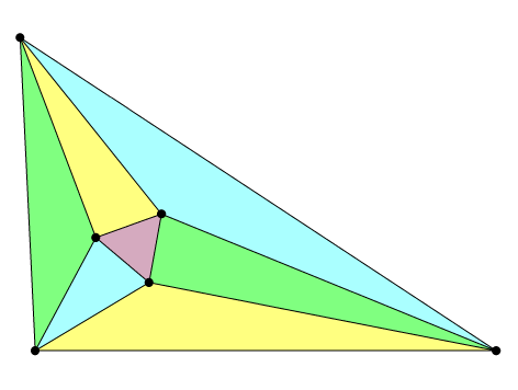
Morley equilateral triangle at the intersection of the trisectors
(from Wikimedia Commons)

In a previous post, I mentioned Morley's miracle: an equilateral triangle appearing at the points of intersection of the angle trisectors of any triangle.

Frank Morley was an excellent teacher and chess player (see some more about him at Pat'sBlog). If he had lived today, I like to think of him having his own blog communicating about his passion for math and chess, submitting his recreational problems. If he hadn't discovered the equilateral triangle at the intersection of trisectors, it's probable that this theorem would still be unknown. Trisection of angles is a controversial subject for research, especially among academia, where it is associated with suspicion of crankiness (see Underwood Dudley's book about trisectors). A pity... because trying to understand how to divide angles is a "natural" question, of which we shouldn't be ashamed, provided that we modestly take into account what has been found by other people.

All the proofs of Morley's theorem that I know of start with a result: an equilateral triangle or a triangle already drawn with its trisectors (see the different proofs referenced on the very complete French site Abracadabri or at the end of Alexander Bogolmony's Cut the Knot site). In this sense, they are backward proofs, which keeps some mystery about the physical origin of the equilateral triangle. I tried something different, a bit similar in spirit to my Archimedes tripling circle: How can we multiply an angle by 3, from which would result a Morley triangle embedded in a triangle of any shape? So here follows an alternative forward proof for Morley's theorem.

Step 1: I start with a circle in which I inscribe an angle α inferior to 60°. The lines are intercepting an arc on the circle.

Step 2: I duplicate the angle by tracing a little circle centered at one of the endpoints of the arc and with radius the chord of that arc. I repeat the same operation to triplicate the angle (see Figure 1).

Step 3: When two circles of equal size and common radius intersect, two equilateral triangles appear, so I draw both of them: Figure 2.

Step 4: I draw supplementary equilateral triangles at both sides, with the help of the intersections of the circles and the outer lines of the triplicate angle, see Figure 3.

Step 5: The magenta colored equilateral triangle is the Morley triangle of the arbitrary triangle we are looking for. The Morley triangle is a pivotal triangle, so the other vertices of the arbitrary triangle can be found through symmetric construction of the initial inscribing circle centered towards the other sides of the Morley triangle, see the red circles at Figure 4.

Step 6: I complete the figure with the triplicated angles β and γ in the red inscribing circles. The sides of the searched triangle are the outer lines of the triplicated angles, see Figure 5.

With this tripling angle construction, we always obtain an equilateral triangle at the intersection of the trisectors of a triangle. When the initial vertex is moved on the initial inscribing circle, all triangle shapes can be generated for any initial angle α between 0 and 60°, which proves the Morley theorem for any triangle.

Archimedes angle trisection or tripling?

Pi-day today, so a nice occasion to write something about circles. π is the ratio between the circles' perimeter (περίμετρος in Greek) and diameter.

In the previous post, I explored some angular tricks using circles. The circle is a key geometrical object when dealing with angles. For example, Archimedes' construction to trisect an angle uses a circle and a straight line with a marked unit. But for clarity's sake, I prefer to draw a set of circles which show how a straight line can mark odd multiples of a unit angle α on intersecting circles, see Figure 1. In that way, it is easier to see how Archimedes' trisection circle relates to the multiplication and division of angles by odd integers, see alternative Figure 2.

This makes me think that Archimedes' angle trisection is in fact the inverse of "Archimedes' angle tripling".

Playing with angles

A few months ago, I prepared this post but didn't feel ready to publish it. It raised more questions than it answered, so I wanted to have a little more background about it. Hopeless wish! There's so much about angles that I don't fully understand. With pi-day approaching, I'm also looking for some inspiration about circles and angles, so I thought publishing might get me in the direction...

I really became aware of the difficulty to divide an angle into three equal angles (a.k.a. angle trisection) some three years ago. It's bloody hard to find general procedures to divide precisely a circular arc into three equal arcs. There are some tricks that are well documented on the web, but you won’t find a simple geometric procedure using only a compass and an unmarked ruler. It has even been "proven" impossible. We only know of some "cheating" tricks like using a marked ruler (for Archimedes' trisection), origami or mechanical tools that will allow you to trisect precisely an angle. And there is an equilateral triangle that appears "by miracle" when you trisect all angles of a triangle, a result found by mathematician Frank Morley (because he himself tried to better understand or crack that impossibility?). So the angle trisection really became to intrigue me and I progressively dug into it.

One of the questions that has obsessed me is : How do we characterize an “Angle”? I’ve already written a post on that question, pointing out the utility of the chord subtending the circular arc of a circle of unit diameter. The measure of this chord is what we call the sine of the subtended angle. It characterizes the angle and it greatly facilitates our way to count angles, for example by progressing stepwise with chords in a circle.

Roughly speaking there are two ways to manipulate angles with circles. Either you use central angles, meaning that you fix the vertex and you radiate towards the circle in order to subtend an arc, or you use inscribed angles, meaning that you put the vertex of the angle on the circle. Figure 1 shows the equivalence between both methods. The central angle of a subtended arc in a circle of radius 1 is equal to the same angle when it is inscribed in a circle of diameter 1. This equivalence between central and inscribed angles is another way of stating that the measure of a central angle is exactly twice the measure of the inscribed angle, the factor 2 expressing the ratio between diameter and radius.

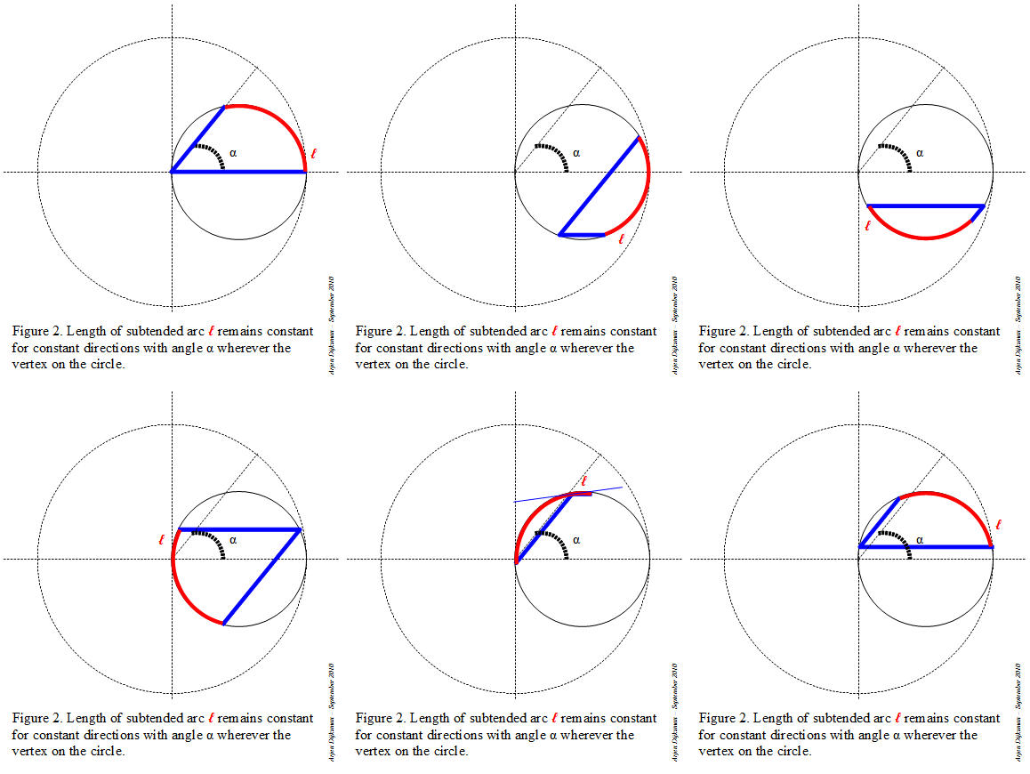
Figure 2 and 3 illustrate some advantages of inscribed angles. You can put the vertex anywhere on the circle: if the subtended circular arc (or its chord) remains constant in length, the angle remains the same. For the case when the vertex is located between the two endpoints of the subtended arc, you have to add the parts at each side of the vertex.

This flexibility of inscribed angles opens possibilities that remain hidden for central angles. If you combine different circles at intersections with straight lines, you’re simply calculating with angles. Figure 4 illustrates an alternative way to count angles. Starting with an angle α inscribed in a circle of unit diameter, if we draw a unit circle symmetric to the chord of the subtended angle, we can read off an angle (α+α) at the other side of the circle. Adding another circle results in an angle (2α+α) at the far side, etc. When the span of the angle exceeds the height of the unit circle, we can use extra circles in order to take over the continuation of the subtended arc (see the angles > 6α on Figure 4. So this simple procedure allows us to read off integer multiples of any angle.

The interesting thing is that wherever we shift a unit circle in this setting, the opposite subtended arcs differ always by an angle amount α, as shown in Figure 5 (in fact the circle needn't be aligned on the axis). So this allows us to add or subtract any angle to another angle.

FQXi essay contest "Is reality digital or analog?"

The third edition of FQXi essay contest is already a success, because there is a growth of 140% in the number of competing essays. There are 161 essays dealing with the question "Is reality digital or analog?" that are waiting for your votes and comments. I have less time to participate in it as for the previous edition on "What's ultimately possible in Physics", but I found it an important question. Important enough to take my pen on vacation and advocate the fact that physical "Reality" must ultimately be accessible to everyone on earth. Reality can be defined in the way we reach universal agreement about it, whether it be analog or digital (I think it will ultimately always be expressed with both concepts of discreteness and continuity: digital and analog).

Some thoughts you'll find in my essay:

"I postulate Reality to be that on which all people can agree"

"Physical reality must be potentially and reproducibly accessible through experiment to any human inhabitant of earth. If it is not, the corresponding statement about reality is biased."

"Some aspects of physics haven’t reached the stadium of universal agreement yet. This is the case for processes at the cosmological scale or at the atomic and nuclear scale, because the rules governing their behavior are not directly part of our everyday experience. We haven’t yet managed to describe all their reality with concepts or words on which everybody can agree. It is the physicist’s job to enlarge the scope of universal agreement about physical reality."
"We will describe anything happening in the submicroscopic world with concepts derived from our macroscopic experience, analogically and digitally. Only then can we come to universal agreement about its reality."

There are 160 other essays. Some are from essay writers whom I already know a little from last year. Unfortunately I won't be able to read more than a few, but I love it to catch up with your ideas, even if I don't always agree with them, probably because I haven't yet got all the information needed to understand your reality. Universal agreement about reality can only be reached if we discuss our ideas openly.

2011 and prime number sieves

I'm a slow blogger. It's already been more than a week that we entered the 2011th year of the Christian era. Interestingly 2011 is a prime number. Many bloggers have mentioned the fact that the number 2011 is also the sum of 11 (a prime number) consecutive primes, see for example at Republic of Math, at Pat'sBlog, at The Math less Traveled, at Lucky's Notes, at the Pattern Connection ... and I apologize to those whom I forget, there must be many more.

I would state the obvious if I said that primes are special numbers. But what makes primality so special? Don Zagier, an eminent specialist, said: Upon looking at these numbers, one has the feeling of being in the presence of one of the inexplicable secrets of creation. That's awesome, isn't it? In antiquity, the Greeks already tried to understand the patterns underpinning the prime numbers. A way to visualize those patterns is through prime number sieves. Eratosthenes is said to have proposed the first sieve, the Eratosthenes sieve. (Hey, have you noticed that Eratosthenes was born 2287 years ago? So we are in year 2287 of the Eratosthenian era. Also a prime number). But there are other sieves. More of that later.

Prime numbers occur in nature in cyclic processes. Imagine that, somewhere in the universe, there's a star with a huge number of planets, all of them having the same orbiting speed. They are numbered from 1 to N, planet n°1 being the inner planet and the diameters of their circular orbits are as following:

• The diameter of planet n°2's orbit is twice the diameter of planet n°1's orbit.
• The diameter of planet n°3's orbit is three times the diameter of planet n°1's orbit.
• The diameter of planet n°4's orbit is four times the diameter of planet n°1's orbit.
• And so on, the unit length being the diameter of planet n°1's orbit, the nth planet has an orbit of diameter n, n being an integer between 1 and N.

Imagine also that at some timestamp zero, all the planets are aligned at the same side of the star (yes I know, this is very improbable, but it's just a thought experiment). We define the orbital period of the first planet as unit time. "Prime times" occur when two and only two planets are aligned on the initial direction with the star: the outer planet than has a prime distance to the star (the closest planet being always planet n°1). I should make an animation to visualize this effect. As making an animation is very time-consuming, I looked for other ways to illustrate this principle and ended up with another sieve: a circle sieve. Instead of drawing concentric circles for the orbits, I shift each circle such that all are tangent at the origin (for example the location of the center of the star, see Figure 1). For each period of a planet, I successively copy its circle and place it tangentially to the right (see Figure 2 for the first periods of planet 1 and 2).

Now, as each planet is orbiting at the same speed, the first alignment along the initial direction will occur at timestamp 2. Planet 1 will have circled twice around the star and planet 2 will have circled once. Circles 1 and 2 touch at abscissa 2. Number 2 is a prime number. The next alignment on the axis will occur for planet 3. Circles 1 and 3 touch at abscissa 3 without circle 2 (see Figure 3). Number 3 is a prime number.

The next alignment will occur for planets 1, 2 and 4. Number 4 is not a prime. But number 5 is prime. We can see that easily if we draw only circles 2 and 3 (leaving out the unit circles), see Figure 4. Prime numbers can only occur at vacant places along the axis. The symmetries that show up along this axis help to design primality tests. Any prime number greater than 3 must be of the form 3*2n±1. This formula is a condensed form of the intersection of odd numbers (noted 2n +1) and non-multiples of 3 (noted 3n+{1,2}) and generates all primes between 3 and 5².

The succession of circles n°5 together with n°2 and 3 sieves out all primes between 5 and 7², see Figure 5.

I let you try it further with circles n°7. You will see patterns with concentric circles become more apparent. I like this geometric variant of Eratosthenes' sieve because symmetries can be caught with the eye and suggest prime generating formulas. For example, I came across two simple prime generating polynomials (which must have been noticed by other people because they are less powerful than Euler's P(n) = n² − n + 41):

n²+9n+1

n²+21n+1

This way of sieving has been described earlier and more extensively by physicist Imre Mikoss. Check his work at "The Prime Numbers Hidden Symmetric Structure and its Relation to the Twin Prime Infinitude and an Improved Prime Number Theorem".

Happy prime year!

Math and Physics: Creative Arts?

My favorite approach towards math is through drawing geometric figures like circles, triangles, squares... They link the mathematical abstraction to the physical reality, whatever that may mean. They help to visualize patterns that may remain hidden when described with symbols. Doodling geometric figures allow digressive exploration of otherwise marked out paths and thus favor creative and curiosity-driven approaches towards math. Although I am not a mathematician, I practice math for my job and as a hobby. I subscribe to views expressed by G.H. Hardy in his Mathematician's Apology

I am interested in mathematics only as a creative art.

or by Paul Halmos in his Mathematics as a Creative Art

Mathematics is far closer to an art than it is to the business of equation-solving.

or by Paul Lockhart in his Mathematician's Lament

I’m just playing. That’s what math  is— wondering, playing, amusing yourself with your imagination.

Interestingly, in these quotes, math could be replaced by physics. Concerning me, it would likewise express my interest in physics. What if all of math and physics could be expressed through art? Well, it should.

Geometric representations of higher degree binomials

A binomial is a mathematical expression with two terms, say x and y. The simplest binomial is the sum of those two terms x+y. Powers of this binomial (x+y)ⁿ are ruled by the so-called binomial theorem, which states that the coefficients of the expansion terms x^py^q are given by the Pascal triangle entries. So we have:
(x+y)⁰ = 1
(x+y)¹ = 1.x + 1.y

(x+y)² = 1.x²+ 2.xy + 1.y²

(x+y)³ = 1.x³+ 3.x²y + 3.xy² + 1.y³

(x+y)⁴ = 1.x⁴+ 4.x³y + 6.x²y² + 4.xy³ + 1.y⁴

and so forth ...

But where do these coefficients come from? You can just be satisfied by the result algebraic calculation, or you could look for geometric representations. For instance, a nice geometric explanation is given at the www.mathaware.org site.

Geometric proof of square binomial (original at The Geometry of the Binomial Theorem, Math Awareness Month site)

Geometric proof of cubic binomial (original at The Geometry of the Binomial Theorem, Math Awareness Month site) 

For the second degree binomial, the Pascal triangle entries emerge naturally as the number of squares or rectangles with area given by the expansion terms x^py^q. For third degree binomials, they emerge as the number of cubes or parallelepipeds with volume given by the expansion terms. And for higher degree binomials, they emerge as the number of hypercubes and hyperparallelepipeds given by the expansion terms, so an Euclidean geometric representation for those higher degree binomials seems impossible.

This suggested impossibility prompted me to have a closer look at geometric representations of binomial expansions. As a matter of fact a number to the fourth power x⁴ is just a number, but it is also a square x⁴ = (x²)². And there is no impossibility in representing numbers and squares geometrically, so the suggested impossibility is only an impossibility along the common line of thought, which sees cubic expansions as volumes. Along another line of thought, which seems to have been unnoticed, cubic expansions can be seen as areas, and then geometric representations of higher degree binomials become possible. The following figures illustrate this fact for the special case where x+y is normalized to 1 (for arbitrary x+y, one just has to rescale the figure each time, the pattern remains the same).

For the binomial (x+y)¹ = 1.x + 1.y, we can divide a unit square into two rectangles, one rectangle of area x and one rectangle of area y, see Figure 1.

For the binomial (x+y)² = 1.x²+ 2.xy + 1.y², we can divide the unit square into two squares, one of area x² and one of area y², plus two rectangles of area xy, see Figure 2.

For the binomial (x+y)³ = 1.x³+ 3.x²y + 3.xy² + 1.y³, we can divide each of the previous squares and rectangles into proportions x and y, giving eight rectangles, one of area x³, one of area y³, plus three rectangles of area x²y and three rectangles of area xy², see Figure 3.

For the binomial (x+y)⁴ = 1.x⁴+ 4.x³y + 6.x²y² + 4.xy³ + 1.y⁴, we can again divide each of the previous squares and rectangles into proportions x and y, giving one square of area x⁴, one of area y⁴, four squares and two rectangles (giving six) of area x²y², four rectangles of area x³y and four rectangles of area xy³, see Figure 4.

And we could go further indefinitely, doodling areas of incrementing powers, just in 2D, without any reference to unintuitive hyperspaces.