Sliding Rectangles and the Lam-Ca Construction

In the quiet elegance of geometric construction, sometimes a simple configuration reveals a profound truth. This post explores one such configuration, part of a legacy left behind by my late Vietnamese friend, Nguyen Tan Tai, who referred to it as the Lam-Ca construction — from the Vietnamese words meaning “do it all.” And that’s exactly what these diagrams aim to do: to explain, prove, and illuminate all at once.

What Nguyen Tan Tai created is more than a diagram: it is a visual proof that brings together trigonometric identities, reciprocal relationships, and the power of constant area.

Click the image or open the interactive Geogebra diagram here.

Unit Diameter Circle Instead of Unit Radius

Most trigonometric constructions begin with a circle with radius 1, where sines and cosines are represented as vertical and horizontal projections of a point on the circle. But in this configuration, the circle has unit diameter.

In a circle of unit diameter:

• The angle α is inscribed.

• The opposite chord has a length equal to sin α.

• For an inscribed right triangle (i.e. with hypotenuse = 1) The adjacent chord has a length equal to cos α.

• The projection of the opposite and adjacent chords on the hypotenuse have respective lengths sin²α and cos²α.

We therefore use chord lengths derived directly from the geometry of the circle. They reflect the sine and cosine values as segments formed within the circle, preserving symmetry and proportions naturally. The squares (blue and red) and rectangles (green and orange) of the upper part of the figure illustrate this nicely. I have already posted this construction in a previous post.

The Insightful Twist: Sliding Rectangles of Constant Area

What Nguyen Tan Tai introduced was an original twist on the classical representation of the inscribed rectangle: instead of constructing squares on the chord segments, he formed rectangles (shown in grey in the lower part of the figure) defined by:

• Left rectangle: one side is sin α, the other is 1/sin α

• Right rectangle: one side is cos α, the other is 1/cos α

The result? Each rectangle has a constant area of exactly 1, even as the angle α changes. In this way we see a whole family of unit-area rectangles. Their lower vertices trace a horizontal line anchored at y = –1. The shape of the rectangle dynamically adapts, while its area remains invariant.

Why This Matters

This construction transforms reciprocal trigonometric identities from abstract formulas into tangible, visual objects. The construction reveals them as side lengths in a dynamic geometry.

This approach:

• Makes reciprocal relationships intuitive

• Shows how geometry can express trigonometry with visual clarity

• Bridges sine and cosine with their multiplicative inverses

• Highlights a rarely explored link between circular geometry and constant-area transformations

The Lam-Ca Perspective

What makes the Lam-Ca construction special is its simplicity: no coordinates, no algebra, just pure geometry. Using circles of unit diameter and basic projections, Nguyen Tan Tai’s approach recovers deep identities from nothing but straightedge-and-compass logic.

This is not just a visual trick. It’s a philosophy: that geometry, when done right, can do it all.

A Quiet Tribute

To our knowledge, this method of constructing unit-area rectangles with sides defined by chord-based trigonometric values and their reciprocals has not been formally documented elsewhere. It stands as a tribute to Nguyen Tan Tai’s creativity and insight—a quietly powerful expression of geometry’s poetic depth.

This visualization is a piece of his legacy, and I’m honored to share it. What if some of the most beautiful trigonometric identities could be seen rather than derived algebraically?

---

In the next post, I’ll extend this same diagram to reveal tripling angle identities like cos(3α) and sin(3α) — all through sliding rectangles and simple symmetry. Stay tuned.

Unveiling Pythagoras: How Circle-Based Area Transformations Reveal the Truth

I recently had a discussion about the Pythagorean theorem and how to understand it better. I realized that the role of the circle as a fundamental element is often underrated. You can hardly find any proof where the right-angled triangle is placed within a circle to support the reasoning. Instead, the triangles are usually presented in a plane without reference. However, when you position the triangle inside a circle, it becomes much easier to visualize how the relationship holds as the right-angle vertex moves along the circle.

The key idea to understand is that in the following image, for a unit square, the green and blue areas are always equal to cos²(α), while the orange and red areas correspond to sin²(α). It is evident that the square, with an area of 1, is the sum of its left and right sections.

By opening the GeoGebra resource [Pythagoras proof in a circle (opens a new tab)], you can slide the right-angle vertex (red point) anywhere along the upper half of the circle. 

Forwards multiplying, backwards dividing

My last post on the Morley triangle theorem got encouraging feedback, namely that it showed the living and breathing side of geometry. Although there are a lot of results discovered in previous, sometimes ancient times, the future of geometry is alike the future of life. You can construct its future in many directions, using different languages, without being constrained by impossibilities which show up on some paths. In case of dead ends, it’s up to us to step back, reexamine the fundamentals, and take another path that has not yet been explored.

One of those geometrical impossibilities which many people know of, is the division of an arbitrary angle by 3, with only a compass and an unmarked ruler. My advice is: don't try it using the geometry you learned at school, you'll be caught in a dead end. Of course, you might try it for some time to get experience with it, experiencing by yourself the hopes and frustrations that generations of mathematical inquirers have felt, but don't expect to break through in this way. In order to bypass the impossibility, you need to step back and try it differently. That's how inquiring minds discovered physical tools or paper folding manners that allow to trisect an angle.

Another way to explore trisection is to reformulate the problem. Dividing an angle is the inverse operation of multiplying an angle. So, if we want to solve problems involving the trisection of an angle, we might first focus on solutions to the problem of tripling an angle. This may sound trivial, so trivial that hardly anyone emphasizes this point. Before learning the operation of division, we should first learn how to multiply. Through multiplication, we advance constructively from a unit towards a product of factors. Once we know how we got that product through multiplication, we can divide backwards the product through factorization.

Multiplying geometrically means generating one length (or surface or volume) from another. If we do this recursively, we get a series of successive powers. For example, with straight lines, using the Thales intercept theorem, we can mark successive powers of a number on lines, see Figure 1. If OA'/OA = x and OA is our unit length and OA' = OB, than you can verify that OB = x, OC = x², OD = x³, OE = x⁴, etc.

So forwards, we multiply each time by x. If we go backwards in the series we divide each time by x and we needn't stop at our initial unit length, but we may divide indefinitely and recursively by x. So the geometric representation of multiplication gives us insight on how to divide an initial length OA by x.

We can do something similar with circular arc lengths. For example, for the recursive doubling of an arc, we can proceed as illustrated in Figure 2.

1. Define a unit arc from an origin O on a circle of center P. Draw also a little circle of diameter OP.
2. If from the endpoint 1 of the unit arc, we draw a radius towards P, it intersects the little circle at the (red) point illustrated on the figure. If we double the (red) chord from O to that (red) point, it will end up at length 2 on the large circle.
3. If from the (red) endpoint 2 of the arc, we draw the (red) radius towards P, it intersects the little circle at the (blue) point illustrated on the figure. If we double the (blue) chord from O to that (blue) point, it will end up at at length 2*2=4 on the large circle.
4. Proceeding further (blue, green, violet...) in the same manner will mark successive powers of 2 on the large circle (as well on the small circle).

If we reverse the direction of this recurrence, we can halve the length of the arc indefinitely. The proof of this recurrence can be given using the isosceles triangles, two sides of which are successive chords.

Update 19 November 2016: the conjectured process below is incorrect. This is not the correct way to multiply angles. It only works for doubling and quadrupling angles (may other powers of 2, I didn't check).

By adapting the geometric configuration of the two circles, we can do the same for the multiplication of an arc by any integer number, forwards. There is no impossibility to multiply an angle by an integer. Reversing the direction of the recurrence, it becomes therefore possible to access to the division of an arc by any integer number, and henceforth any rational number. As food for thought, the beginning of the conjectured process is illustrated in Figure 3.

1. Draw a circle of diameter QP.
2. A circle of center P and with radius smaller than QP defines the origin of the arc at one of their intersections O.
3. Define a unit arc from origin O on the circle of center P.
4. If from endpoint 1 of the unit arc, we draw a radius towards P, it intersects the other circle at the (red) point illustrated on the figure. If we prolongate the (red) chord from Q to the (red) point, it will end up at length x on the arc.
5. If from (red) endpoint x of the arc, we draw the (red) radius towards P, it intersects the other circle at the (blue) point illustrated on the figure. If we prolongate the (blue) chord from Q to that (blue) point, it will end up at length x*x=x² on the arc.
6. Proceeding further (blue, green...) in the same manner will mark successive powers of x on the circle.

Morley triangle derived from the tripling of an angle

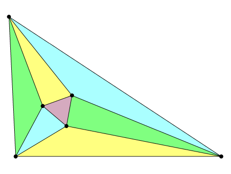
Morley equilateral triangle at the intersection of the trisectors
(from Wikimedia Commons)

In a previous post, I mentioned Morley's miracle: an equilateral triangle appearing at the points of intersection of the angle trisectors of any triangle.

Frank Morley was an excellent teacher and chess player (see some more about him at Pat'sBlog). If he had lived today, I like to think of him having his own blog communicating about his passion for math and chess, submitting his recreational problems. If he hadn't discovered the equilateral triangle at the intersection of trisectors, it's probable that this theorem would still be unknown. Trisection of angles is a controversial subject for research, especially among academia, where it is associated with suspicion of crankiness (see Underwood Dudley's book about trisectors). A pity... because trying to understand how to divide angles is a "natural" question, of which we shouldn't be ashamed, provided that we modestly take into account what has been found by other people.

All the proofs of Morley's theorem that I know of start with a result: an equilateral triangle or a triangle already drawn with its trisectors (see the different proofs referenced on the very complete French site Abracadabri or at the end of Alexander Bogolmony's Cut the Knot site). In this sense, they are backward proofs, which keeps some mystery about the physical origin of the equilateral triangle. I tried something different, a bit similar in spirit to my Archimedes tripling circle: How can we multiply an angle by 3, from which would result a Morley triangle embedded in a triangle of any shape? So here follows an alternative forward proof for Morley's theorem.

Step 1: I start with a circle in which I inscribe an angle α inferior to 60°. The lines are intercepting an arc on the circle.

Step 2: I duplicate the angle by tracing a little circle centered at one of the endpoints of the arc and with radius the chord of that arc. I repeat the same operation to triplicate the angle (see Figure 1).

Step 3: When two circles of equal size and common radius intersect, two equilateral triangles appear, so I draw both of them: Figure 2.

Step 4: I draw supplementary equilateral triangles at both sides, with the help of the intersections of the circles and the outer lines of the triplicate angle, see Figure 3.

Step 5: The magenta colored equilateral triangle is the Morley triangle of the arbitrary triangle we are looking for. The Morley triangle is a pivotal triangle, so the other vertices of the arbitrary triangle can be found through symmetric construction of the initial inscribing circle centered towards the other sides of the Morley triangle, see the red circles at Figure 4.

Step 6: I complete the figure with the triplicated angles β and γ in the red inscribing circles. The sides of the searched triangle are the outer lines of the triplicated angles, see Figure 5.

With this tripling angle construction, we always obtain an equilateral triangle at the intersection of the trisectors of a triangle. When the initial vertex is moved on the initial inscribing circle, all triangle shapes can be generated for any initial angle α between 0 and 60°, which proves the Morley theorem for any triangle.

Playing with angles

A few months ago, I prepared this post but didn't feel ready to publish it. It raised more questions than it answered, so I wanted to have a little more background about it. Hopeless wish! There's so much about angles that I don't fully understand. With pi-day approaching, I'm also looking for some inspiration about circles and angles, so I thought publishing might get me in the direction...

I really became aware of the difficulty to divide an angle into three equal angles (a.k.a. angle trisection) some three years ago. It's bloody hard to find general procedures to divide precisely a circular arc into three equal arcs. There are some tricks that are well documented on the web, but you won’t find a simple geometric procedure using only a compass and an unmarked ruler. It has even been "proven" impossible. We only know of some "cheating" tricks like using a marked ruler (for Archimedes' trisection), origami or mechanical tools that will allow you to trisect precisely an angle. And there is an equilateral triangle that appears "by miracle" when you trisect all angles of a triangle, a result found by mathematician Frank Morley (because he himself tried to better understand or crack that impossibility?). So the angle trisection really became to intrigue me and I progressively dug into it.

One of the questions that has obsessed me is : How do we characterize an “Angle”? I’ve already written a post on that question, pointing out the utility of the chord subtending the circular arc of a circle of unit diameter. The measure of this chord is what we call the sine of the subtended angle. It characterizes the angle and it greatly facilitates our way to count angles, for example by progressing stepwise with chords in a circle.

Roughly speaking there are two ways to manipulate angles with circles. Either you use central angles, meaning that you fix the vertex and you radiate towards the circle in order to subtend an arc, or you use inscribed angles, meaning that you put the vertex of the angle on the circle. Figure 1 shows the equivalence between both methods. The central angle of a subtended arc in a circle of radius 1 is equal to the same angle when it is inscribed in a circle of diameter 1. This equivalence between central and inscribed angles is another way of stating that the measure of a central angle is exactly twice the measure of the inscribed angle, the factor 2 expressing the ratio between diameter and radius.

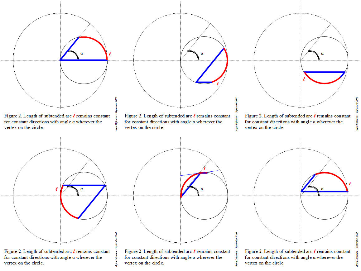
Figure 2 and 3 illustrate some advantages of inscribed angles. You can put the vertex anywhere on the circle: if the subtended circular arc (or its chord) remains constant in length, the angle remains the same. For the case when the vertex is located between the two endpoints of the subtended arc, you have to add the parts at each side of the vertex.

This flexibility of inscribed angles opens possibilities that remain hidden for central angles. If you combine different circles at intersections with straight lines, you’re simply calculating with angles. Figure 4 illustrates an alternative way to count angles. Starting with an angle α inscribed in a circle of unit diameter, if we draw a unit circle symmetric to the chord of the subtended angle, we can read off an angle (α+α) at the other side of the circle. Adding another circle results in an angle (2α+α) at the far side, etc. When the span of the angle exceeds the height of the unit circle, we can use extra circles in order to take over the continuation of the subtended arc (see the angles > 6α on Figure 4. So this simple procedure allows us to read off integer multiples of any angle.

The interesting thing is that wherever we shift a unit circle in this setting, the opposite subtended arcs differ always by an angle amount α, as shown in Figure 5 (in fact the circle needn't be aligned on the axis). So this allows us to add or subtract any angle to another angle.

Geometric representations of higher degree binomials

A binomial is a mathematical expression with two terms, say x and y. The simplest binomial is the sum of those two terms x+y. Powers of this binomial (x+y)ⁿ are ruled by the so-called binomial theorem, which states that the coefficients of the expansion terms x^py^q are given by the Pascal triangle entries. So we have:
(x+y)⁰ = 1
(x+y)¹ = 1.x + 1.y

(x+y)² = 1.x²+ 2.xy + 1.y²

(x+y)³ = 1.x³+ 3.x²y + 3.xy² + 1.y³

(x+y)⁴ = 1.x⁴+ 4.x³y + 6.x²y² + 4.xy³ + 1.y⁴

and so forth ...

But where do these coefficients come from? You can just be satisfied by the result algebraic calculation, or you could look for geometric representations. For instance, a nice geometric explanation is given at the www.mathaware.org site.

Geometric proof of square binomial (original at The Geometry of the Binomial Theorem, Math Awareness Month site)

Geometric proof of cubic binomial (original at The Geometry of the Binomial Theorem, Math Awareness Month site) 

For the second degree binomial, the Pascal triangle entries emerge naturally as the number of squares or rectangles with area given by the expansion terms x^py^q. For third degree binomials, they emerge as the number of cubes or parallelepipeds with volume given by the expansion terms. And for higher degree binomials, they emerge as the number of hypercubes and hyperparallelepipeds given by the expansion terms, so an Euclidean geometric representation for those higher degree binomials seems impossible.

This suggested impossibility prompted me to have a closer look at geometric representations of binomial expansions. As a matter of fact a number to the fourth power x⁴ is just a number, but it is also a square x⁴ = (x²)². And there is no impossibility in representing numbers and squares geometrically, so the suggested impossibility is only an impossibility along the common line of thought, which sees cubic expansions as volumes. Along another line of thought, which seems to have been unnoticed, cubic expansions can be seen as areas, and then geometric representations of higher degree binomials become possible. The following figures illustrate this fact for the special case where x+y is normalized to 1 (for arbitrary x+y, one just has to rescale the figure each time, the pattern remains the same).

For the binomial (x+y)¹ = 1.x + 1.y, we can divide a unit square into two rectangles, one rectangle of area x and one rectangle of area y, see Figure 1.

For the binomial (x+y)² = 1.x²+ 2.xy + 1.y², we can divide the unit square into two squares, one of area x² and one of area y², plus two rectangles of area xy, see Figure 2.

For the binomial (x+y)³ = 1.x³+ 3.x²y + 3.xy² + 1.y³, we can divide each of the previous squares and rectangles into proportions x and y, giving eight rectangles, one of area x³, one of area y³, plus three rectangles of area x²y and three rectangles of area xy², see Figure 3.

For the binomial (x+y)⁴ = 1.x⁴+ 4.x³y + 6.x²y² + 4.xy³ + 1.y⁴, we can again divide each of the previous squares and rectangles into proportions x and y, giving one square of area x⁴, one of area y⁴, four squares and two rectangles (giving six) of area x²y², four rectangles of area x³y and four rectangles of area xy³, see Figure 4.

And we could go further indefinitely, doodling areas of incrementing powers, just in 2D, without any reference to unintuitive hyperspaces.

Alternative Pythagorean quadruples and other extensions to Pythagoras theorem

The vertices of an arbitrary triangle can be disposed onto two concentric circles such that the base is the diameter of the first circle (which I call the base circle) and the opposite vertex is on the second circle (which I call the leg circle). As there are three bases, there are generally three ways to arrange this setting. I mentioned in my preceding post that we can apply the Pythagorean-like relation a²+b²=c²±2t² to this triangle, where c is its base, a and b are the legs and t is the tangent to the inner circle emanating from the outer circle. For clarity, I reproduce an illustrative figure from my preceding post, for the case where the inner circle is the base circle.

Now, like for the classical Pythagoras relation, there are many features that can be investigated regarding this alternative relation. For example, I would like to better understand the relation of this 2D formula with the Cartesian 3D variant of Pythagoras: x²+y²+z²=d², which is analogous to the case where the leg circle is smaller than the base circle (see Figure 5c of preceding post). Another interesting aspect is the fact that the square of the tangent t² (multiplied by π) determines the area of the annular ring delimited by the base and the leg circles, as stated by Mamikon Mnatsakanian. This fact offers possibilities for areal representations of the squares or circles related to the sides of the arbitrary triangle, like we are acquainted to do with the squares related to the sides of a right triangle. Also, what would be interesting to develop is its relation with the law of cosines (as noticed by Pat Ballew) and the angle subtended by sides a and b. I guess this will leave enough stuff for future posts or conversations, or even papers in specialized journals.

As a conclusion, let me mention Pythagorean numerological features which provide stuff for entertaining puzzles. Maybe you know the Pythagorean triples, those sets of integer numbers (n,m,l) that verify n²+m²=l² and of which (3,4,5) is the simplest instance. The 3D Pythagoras relation allows an extension to Pythagorean quadruples, sets of integer numbers (n,m,l,k) that satisfy n²+m²+l²=k² and of which (1,2,2,3) is the simplest instance. I couldn't resist to look for some integer quadruples that satisfy a²+b²=c²+2t². Among them I found two nice quadruples with successive a,b,c :

(7,8,9,4) for which 7² + 8² = 9² + 2 × 4² = 113

(35,36,37,24) for which 35² + 36² = 37² + 2 × 24² = 2521

A Pythagorean relation for any triangle?

Physics makes extensive use of the Pythagorean law relating the squares of the sides of a right triangle. The well-known a² + b² = c² relation is of special interest for the determination of distances and lengths of vectors, but also for energy conservation laws and Lorentz transformations. There are various relations that resemble the Pythagoras law, but none of them seems to have the usefulness of Pythagoras’ original one, as well as the “beauty” originating from its sole quadratic terms. When the vertex opposite to the hypotenuse runs on the circle determined by the right triangle, we have the Pythagoras relation illustrated in Figure 1.

Some time ago, I was made aware of another interesting Pythagorean law, discovered by Nguyen Tan Tai and which I mentioned in a previous post. For any triangle with sides a, b and c, if the vertex opposite to the base (say c) runs on any fixed circle centered at the center of c, we have the relation:

a² + b² = c² + constant

In order to have a better understanding of this quadratic relation, I tried to re-derive it in my own mental representation. I will call the fixed circle with the running vertex C the “leg circle”, because it is determined by the vertex that is common to legs AC and BC of the triangle (see Figure 2).

When the leg circle is larger than the base circle, the legs AC and BC intersect the base circle and we can decompose the arbitrary triangle into two right triangles, for example as illustrated in Figure 3, the right triangles ABD and BCD.

With the Pythagoras relation we than have:

AC² + BC² = (AD + CD)² + BC²
= (AD² + CD² + 2.AD.CD) + (BD² + CD²)
= AD² + BD² + 2.CD² + 2.AD.CD
= (AD² + BD²) + 2.(AD + CD).CD
= AB² + 2.AC.CD

But the product AC.CD is the power of point C with respect to the base circle, i.e. for every point C on the leg circle, AC.CD is constant and equal to the square of the tangent ray CT (see Figure 4).


If we use another notation, AC = a, BC = b, AB = c and CT = t, the relation becomes a nice equation with only quadratic terms:

a² + b² = c² + t² + t²

One can verify that if the leg circle has same size as the base circle, we retrieve the original Pythagoras relation :

a² + b² = c²

And if the leg circle is smaller than the base circle, we have:

a² + b² + t² + t² = c²

where t is now the tangent ray to the leg circle emanating from any point of the base circle.

We thus have a Pythagoras-like relation for any triangle given its base and leg circles, as illustrated by Figures 5a, 5b and 5c.

Lost theorem about angular proportions

Last week, I came across a so called missing theorem about angular proportions in a triangle, discovered (or rediscovered) by Leon Romain. This triangle construction is presented by user Linelites on youtube.

For such a "Romain triangle", the missing theorem states that, if one of the inner angles is twice another inner angle, one has the property a² = bc +c², where a, b and c are outlined in Figure 1.

The sine chord pattern presented in the Teaching sine function with spaghetti provides helpful insights for the missing theorem. In this pattern, all angles at the intersection of chords are integer multiples of a chosen unit angle or its complement, modulo 90°. All segment lengths in this pattern can therefore be written as sums or differences of cosine and sine products and ratios of that angle. Figure 2 pictures some measures of sine chords in a circle of unit diameter, for an arbitrary angle θ.

Figure 3 shows a Romain triangle for angle α in this pattern. There are numerous other Romain triangles in this pattern. Can you figure them out? With the help of the measures pictured in Figure 2, one can follow visually the elements of a proof for the missing theorem.

Side b is the sine of the chosen angle θ (Figure 4):

b = sinθ

Side c times sin3θ equals b times sinθ (Figure 5):

c = sin²θ/sin3θ

Side a equals b cosθ minus c cos3θ (Figure 6)

a = sinθ cosθ - sin²θ cos3θ /sin3θ

Working out a² and bc +c², one finds that they are both equal to 2 sin²θ cosθ / sin3θ.

The interesting thing is that the sine chord pattern hosts plenty of "missing theorems" about angular proportions, which are only waiting to be (re)discovered.

______________________
Update (June 7, 2010): I corrected Figure 6, which held a wrong term.

Teaching sine function with spaghetti

Sine functions appear everywhere in physics and mathematics. This seems to be related to the circular symmetry of space and to the periodic behavior of dynamical processes. The usual definition is that the sine of an angle is the ratio of the length of the opposite side to the length of the hypotenuse in a right triangle (definition at wikipedia). The sine is also often represented as the ordinate of a point running on a unit circle centered at the origin. Any right triangle can be put in that setting. The length of the blue segment on Figure 1 illustrates this definition for an arbitrary angle α, in a circle of unit radius.

It is of interest to have in mind other geometric representations of the sine function. This helps to associate figures with sine and cosine operations or identities. The red segment in Figure 1 shows such an alternative representation, because the sine is also a chord of a circle of unit diameter. When we increment the angle by steps α, one endpoint of the chord advances on the little circle, while the other endpoint remains fixed at the origin, as illustrated by the animation in Figure 2.

When it represents the sine of angle α, the chord in the little circle spans an angle 2α. It is therefore a direct way to the angle multiplication and division by 2. Moreover, the endpoints of this chord can be placed two by two in any other direction on this circle. This enables one to find other variations on the recurrence pattern of the angle in the circle. During one of my circle drawing sessions, I was surprised by the stepwise zigzagging pattern of Figure 3.

Teaching the sine function with this zigzag pattern is particularly suited for daily life situations. Children like it, especially when you explain it at the table.

Keeping track of the circle for integral representations of π

The fundamental constant π is characterized in many ways. Historically, it all began from tentative measurements of the circle's perimeter or area and gradually shifted into more advanced mathematics, in such a way that the link between the circle and modern characterizations of π faded away, see for example the formulas presented at Wolfram MathWorld or Wikipedia.

In the preceding posts, I mentioned infinite products as approximations for π. These may be seen geometrically as exhaustion methods, where the area of a polygon approaches the circular area alternately from above, from below, from above, from below, etc.

There are also integral representations of pi. In such integral representations, π appears in the quantitative value of the integral of a mathematical function. Visually, this is often represented as the area delimited by the bounds of the function. However, the relation with the circle is lost, when viewed under Cartesian coordinates. For example, the graph of the simplest instance of the Cauchy-Lorentz distribution, f(x)=1/(1+x²), "has nothing at all to do with circles or geometry in any obvious way" as quoted from last Pi-day Sunday function from Matt Springer's Built on Facts blog.

In order to view the role of the circle in integral representations of π, we need to switch to alternative ways to visualize math functions. As an example, let's take the constant function y=f(x)=2. The function f maps an element x from a domain to the element y of the target. In this case, for every x, the target y has the constant value 2. With Cartesian coordinates, we are used to represent this function as a horizontal straight line, like in Figure 1a (click on the figure to view it enlarged). If however we write it as R=f(r)=2, where the function f maps any circle of radius r of the domain to a target circle of radius R=2, the same function can be viewed as a circle of constant radius, like in Figure 1b. So the same function f can be equally well viewed as a straight line or as a circle (x, y, r or R are only dummy variables).

Now if we take another example, the linear function, y=f(x)=2x, we are often used to view it in Cartesian coordinates as a straight line with slope 2, like in Figure 1c. In the circular representation R=f(r)=2r, this works however differently. Because we are relating circles of the input domain to other circles of the target, for each circle of radius r, we need to draw the target circle of radius 2r. A single line won't do. For one value of r, we need to draw two circles. If we use blue circles for elements of the input domain and red circles for elements of the target, we could visualize it for successive values of r as an animation like in Figure 1d. In that way, we view the progression of the target circle as the input circle becomes larger.

Unlike the Cartesian representation which shows the progression of a function in a static graph, this circular representation needs a dynamic or recurrent process to get grip of the progression of the function. Therefore it isn't very adapted for illustrations in print media. On the other hand, it has the advantage of keeping track of the geometrical form of the circle. And that's exactly what we need in order to perceive the circular nature when π shows up in mathematical functions. The relation of the integral of the Cauchy-Lorentz distribution f(r)=1/(1+r²) with the circle can then be seen with the help of the geometric counterparts of arithmetic operations like addition, squaring and dividing. A convenient procedure is illustrated in the successive steps of Figure 2.

Step 1. Draw the input circle of radius r and the reference circle of radius unity.

Step 2. Determine r².

Step 3. Add 1 to r².

Step 4. Invert (1+r²). We now have the target circle of radius R=1/(1+r²).

Step 5. Find the target ring related to the input ring ranging over [r, r + dr]. This yields a ring of width dr/(1+r²). The location of this ring depends on the relative progression rates of r and r² (I've not yet found a straightforward explanation for this determination).

Step 6. Integrate dr/(1+r²) for r running over all space. For r becoming larger and larger, the summed area tends towards the area of a circle of radius 1. For the positive half plane, this corresponds to the π/2 value found analytically.

The tricky step seems to be the way how to relate the progression between r and 1/(1+r²) in steps 5 and 6. One can verify for example the value of the integral at intermediate steps. For the integral from r=0 to 1, the value in the positive half plane must be π/4, which can be verified on the figure below.

In order to gain more insight on π, it could be of interest to develop skills for this circular representation.